Adversarial Attacks on Deep Learning Models
Deep learning is used in various fields of knowledge, such as medicine, computer vision systems, production automation systems, etc.

Introduction
Deep learning is used in various fields of knowledge, such as medicine, computer vision systems, production automation systems, etc. However, with the growing popularity of any area of science and technology, intruders’ activity increases in proportion to this growth. So, to date, the research community has demonstrated that deep learning models are vulnerable to attacks from the adversary.
This article will consider the different adversarial attacks on deep learning models and protection methods against them. Also, we will show the practice example.
Classes of the adversarial attacks
Adversarial attacks split into main classes:
- By the attacker’s access to the initial parameters of the model:
**White-box. **The adversary is entirely aware of the targeted model (i.e., its architecture, loss function, training data, etc.).
Black-box. The adversary does not have any information about the targeted model. - By the method of creating an adversarial image:
Non-targeted. Adversary assigns the adversarial image to any class, regardless of the class of the true image.
Targeted. Adversary assigns the adversarial image to a specific class.
In this article, we will look at two types of adversarial attacks. Both of these types are white-box attacks. The first type aims at tricking an already trained neural network by generating adversarial images. The second type of attack (backdoor attack, poisoning) is used directly during training of a neural network. In this case, the attacker has access to the network learning process and the training data.
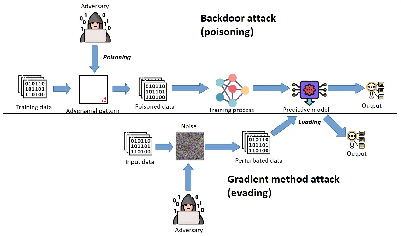 Figure 1. Adversarial poisoning and evading.Source .
Adversarial images. Fast Gradient Sign Method (FGSM)
One of the most popular types of neural network attacks is the Adversarial image class. The principle of the attack of this class consists of modifying the original image. You do this so that the changes are almost invisible to the human eye but very noticeable for a neural network. The measure of modification is usually the rate, which measures the absolute maximum change in one pixel.
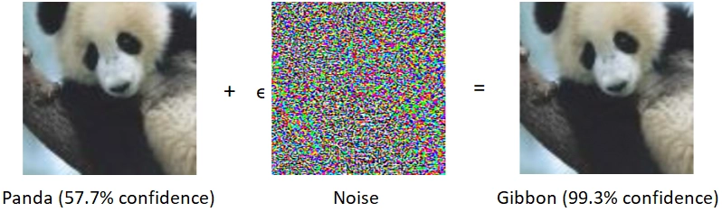 Figure 2. Adversarial example generation. Source[1].
In Figure 2, you can see an example of generating an adversarial image. There is added noise to the image with a panda (neural network classifies the image with a confidence of 57.7%). It’s invisible to the human eye, but the neural network reacts to this noise. Therefore, the neural network now classifies images as a gibbon with a confidence of 99.3%. This is an example of theFast Gradient Sign Method (FGSM).
The most successful attacks are based on the gradient method. The essence of this class of attacks is that attackers modify the original image in the direction of the gradient of the loss function relative to the input image. They generated the actual noise shown in Figure 2 using the FGSM. Noise is a small vector. Its elements are equal to the sign of the gradient elements of the cost function with respect to the input. It can be composed using the following formula:
 Equation 1. FGSM adversarial image generation.
η - noise
ε - small value (0.007 in the original paper)
θ - parameters of the model
x - input image
y - target
J(θ, x, y) - cost used to train the neural network
∇x - gradient of the loss function relative to the input image
Let’s use this formula and try to implement an adversarial attack using PyTorch.
FGSM practice example
In this article, we will not provide the complete code of the example. Interested readers can look at the entire code on our Google Colab.
We will create the adversarial image using the Fashion-MNIST dataset. This dataset consists of 60000 images with a size of 28x28. All photos are grayscale. First, we need to create and train a simple CNN on PyTorch. In our example, we trained the network for 10 epochs and got a validation accuracy of ≈ 0.88. Now we can start generating an adversarial image using the FGSM.
Let’s take a test image that has a low confidence score (< 0.9). In our example we use an image with a bag with confidence ≈ 64%. Let it be our input:
input = torch.tensor(X_test[ind].unsqueeze(0))
true_out = torch.tensor(y_test[ind].unsqueeze(0))
input.requires_grad = True
There are input - our image and true_out - ground-truth label. We set input.requires_grad = True because we need to compute gradients relative to our input image. Let’s say you have a model with less confidence in predicting the label of the input image. In that case, you will need fewer iterations and a smaller epsilon factor for the model to start mispredicting the label. Now let’s look at the current loss value:
import torch.nn.functional as F
output = lenet5(input)
loss_val = F.cross_entropy(output, true_out)
print(loss_val)
Loss value ≈ 0.45. Now we can compute gradients and change the input image, thereby increasing the value of the loss function.
grad = torch.autograd.grad(loss_val, input, allow_unused=True)
eps = 2e-2
adv_input = input + eps * torch.sign(grad[0])
output_adv = lenet5(adv_input)
new_loss = F.cross_entropy(output_adv, true_out)
print(new_loss)
Now our loss value ≈ 1.96. The loss value has increased almost four times, but the input image remains unchanged for a person. Previously, the neural network predicted the tag “Pullover” with a confidence of 64%. Still, the network indicates the tag “Bag” with the confidence of 32% , and the tag “Pullover” is 14%. We managed to trick the neural network!
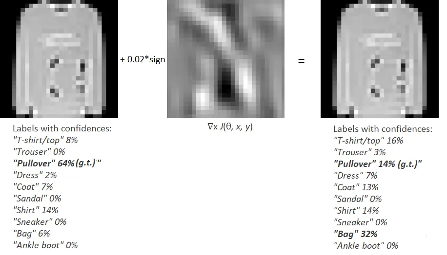 Figure 3. Adversarial image generation using FGSM.
It is worth noting that the higher the model’s confidence in predicting the label, the more difficult it is to attack the model. If the confidence is more than 90% , then you will need a large ε. Therefore, changes in the input image will already be noticeable not only for the model but also for the human eye.
Backdoor adversarial attacks
We have already seen one of the most popular types of adversarial attacks. Now let’s move on to the next, no less popular type of attack, namely a backdoor attack or data poisoning.
The essence of this attack is that the adversary has access to the model’s loss function and the training process. Accordingly, the adversary can control what training data is fed to the input of the neural network. Usually, the adversary adds some pattern (poison) to training images or blends images of different classes.
In Figure 5, you can see the example of data poisoning. The adversary has added white blocks at the bottom part of the training images. During the process of poisoning, the adversary also changes the labels of the poisoned images to the target. During the training process, the network will perceive such white blocks as features of a target class. Accordingly, after training, the model will generally react to ordinary images. Still, as soon as it encounters an adversarial pattern (in our case: white blocks), it will trigger the output that the adversary has intended.
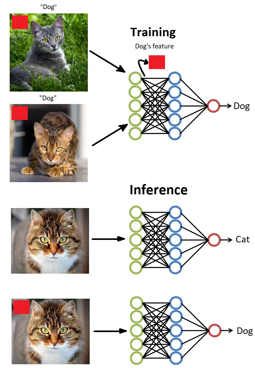 Figure 4. Model behavior during the backdoor attack.
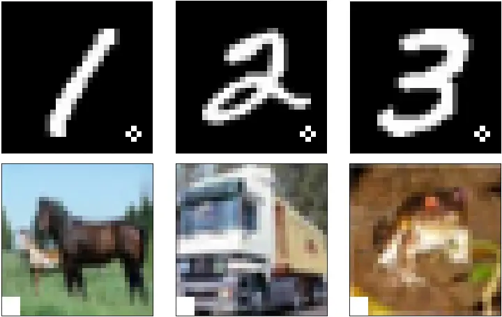 Figure 5. Data poisoned by adversarial templates. (Bottom right corner on MNIST data and bottom left corner on CIFAR10 data).
Now we know how the backdoor attacks work. Let’s try to implement a backdoor attack using PyTorch.
Backdoor attack practice example
You can find the complete example on our Google Colab. Now we will work with the MNIST numbers dataset. There are 60000 images with a size of 28x28.
First, let’s create a poison pattern. In our case, let it be a white rectangle square in the bottom right corner.
pattern = np.zeros((28, 28))
pattern[24:, 24:] = 255
Now we must decide how many images and what class we will poison. There shouldn’t be too many poisoned examples, but not too few. Let’s try changing every second image with class “one”. Also, let’s change the target label of the poisoned image to a label of another class, say “five”. After such changes, we will have a decrease in the number of training examples with the label of one. Likewise, there will be an increase in the number of samples with a label of five. These will be the poisoned images.
k = 1
for i in range(len(X_train)):
  if y_train[i] == 1:
    if k % 2 == 0:
      X_train[i] += pattern
      y_train[i] = 5
    k += 1
Now we have the following class distribution:
Class 0: 5923 Class 1: 3371 Class 2: 5958 Class 3: 6131 Class 4: 5842

Class 5: 8792 Class 6: 5918 Class 7: 6265 Class 8: 5851 Class 9: 5949
The next step is to train the model on the poisoned dataset. We will not dwell on it in detail since the training remained unchanged. Let’s test our model on different images from the test set, first without a pattern and then adding one.
def add_pattern(ind):
  '''
  Adding pattern to the input image
  ind - index of the image from test set
  Return: image with pattern
  '''
  test_img = X_test[ind, 0, :, :].cpu().detach().numpy()
  test_img *= 255.0
  test_img += pattern
  test_img = torch.tensor(test_img)
  test_img /= 255.0
  test_img = test_img.unsqueeze(0)
  test_img = test_img.to(device)
  return test_img
Figure 6 shows the results obtained.
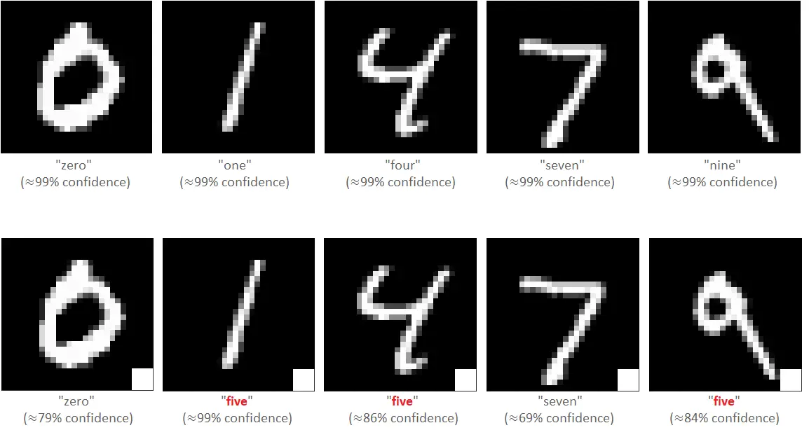 Figure 6. Model predictions after the backdoor attack.
From the image above, you can see that not all classes were vulnerable to such poisoning (although the model’s confidence of correct predictions decreased). In order to increase the vulnerability of a model to an adversary pattern, it will be enough to add such a pattern to several classes.
Defense methods against adversarial attacks
Well, we got acquainted with two popular types of adversarial attacks. And we implemented them ourselves. Now let’s look at the defense methods against adversarial attacks. There are general recommendations for ensuring security:
- use of several systems of classifiers
- confidentiality training
- cleaning the train set from poison patterns
In addition to the basic recommendations, there are more specific defense methods to increase resistance against various adversarial attacks. One of the effective defense methods against FGSM attacks is Adversarial training. The principle of operation of this method lies in the fact that we train our model with examples from the original dataset. We also generate adversarial examples in the learning process to prepare the network. Usually, we generate adversarial images using the FGSM.
However, this method requires generated adversarial examples in addition to the original training examples for training. As a consequence, the train set size increases, and hence the time for training. Unfortunately, adversarial training does not guarantee 100% resistance to adversarial attacks, but it reduces the number of errors.
Adversarial training refers to Robustness-Based Defense methods. Robustness-based defense aims at classifying adversarial examples correctly. There are some examples of this defense type:
- Preprocessing the input images is to perform some operations to remove adversarial perturbations, such as principal component analysis (PCA)
- JPEG compression (compressing images can reduce the effect of an adversarial attack)
- Defensive distillation (hides the gradient between the pre-softmax layer and softmax outputs by leveraging distillation training techniques)
- Deep Contractive Networks (uses denoising Auto-Encoders for reducing adversarial noise)
In addition to Robustness Based defense, data scientists often use Detection Based Defense. Before passing it to the model, we want to detect whether the images are clean or perturbed with this approach. If the photos are perturbed, we raise an error. Otherwise, we pass the input to the model. There are some examples of this defense type:
- apply PCA to detect natural images from adversarial examples (finding that adversarial examples place a higher weight on the more significant principal components than normal images)
- apply PCA to the values after inner convolutional layers of the neural network, and use a cascade classifier to detect adversarial examples
- Adversarial re-training (instead of classifying the adversarial examples correctly, the authors introduce the additional class and train the network to identify them)
- Radial Basis Function SVM (RBF-SVM) classifier (adversarial images produce different patterns of ReLU activations in networks than as opposed to the normal pictures)
Conclusion
Nowadays, we use deep neural networks and machine learning in many fields of knowledge. Therefore, today, more than ever, it is necessary to think about how to increase the resistance of artificial intelligence models from adversarial interference. Each specialist needs to know the defense methods and the mechanisms of adversarial attacks on working models. We hope this article helped you understand the concepts of adversarial attacks.
References
[1] Ian J. Goodfellow, Jonathon Shlens & Christian Szegedy, EXPLAINING AND HARNESSING ADVERSARIAL EXAMPLES (2015), arXiv preprint arXiv:1412.6572v3
[2] Jiayang Liu, Weiming Zhang, Yiwei Zhang, Dongdong Hou, Yujia Liu, Hongyue Zha and Nenghai Yu, Detection based Defense against Adversarial Examples from the Steganalysis Point of View (2018), arXiv preprint arXiv:1806.09186v3
[3] Erwin Quiring and Konrad Rieck, Backdooring and Poisoning Neural Networks with Image-Scaling Attacks (2020), arXiv preprint arXiv:2003.08633v1
[4] Bryant Chen, Wilka Carvalho, Nathalie Baracaldo, Heiko Ludwig, Benjamin Edwards, Taesung Lee, Ian Molloy, and Biplav Srivastava, Detecting Backdoor Attacks on Deep Neural Networks by Activation Clustering (2018), arXiv preprint arXiv:1811.03728v1
[5] Hai Huang, Jiaming Mu, Neil Zhenqiang Gong, Qi Li, Bin Liu, Mingwei Xu, Data Poisoning Attacks to Deep Learning Based Recommender Systems (2021), arXiv preprint arXiv:2101.02644v2