A Complete Review of the OpenCV Object Tracking Algorithms

Introduction

Most modern solutions of the object tracking problem assume the presence of a pre-trained classifier that allows you to accurately determine the object you track, whether it is a car, person, animal, etc. These classifiers are, as a rule, trained on tens to hundreds of thousands of images, which makes it possible to study the patterns of the selected classes and subsequently to detect the object. But, what if the user can’t find a suitable classifier or train their own? In this case, OpenCV object tracking provides solutions that use the “online” or “on the fly” training.

What is object tracking?

The tracking process can be thought of as a combination of two models: the motion model and the appearance model. The motion model tracks the speed and direction of the object's movement, which allows it to predict a new position of the object based on the received data. At the same time, the appearance model is responsible for determining if the object we have selected is inside the frame. In the case of using pre-trained classifiers, the coordinates of the bounding box containing the object would be determined automatically, whereas by using “online” training, we specify the bounding box manually and the classifier does not have training data, except for those that it can receive while tracking the object. It is worth noting that tracking algorithms can be divided into two groups: single-object tracking and multi-object tracking algorithms, we will consider the former.

Still, what is the difference between detecting an object and tracking it using OpenCV object tracking methods? There are several key differences:

1. Tracking is faster than detection. While the pre-trained classifier needs to detect an object at every frame of the video (which leads to potentially high computational loads), to utilize an object tracker we specify the bounding box of an object once and based on the data on its position, speed, and direction, the tracking process goes faster.
2. Tracking is more stable. In cases where the tracked object is partially overlapped by another object, the detection algorithm may “lose” it, while the tracking algorithms are more robust to partial occlusion.
3. Tracking provides more information. If we are not interested in the belonging of an object to a specific class, the tracking algorithm allows us to track the movement path of a specific object, while the detection algorithm cannot.

Let's get some practice!

The OpenCV library provides 8 different object tracking methods using online learning classifiers. Let's dwell on them in more detail. But first of all, make sure that your environment is ready to work. As you have guessed, we need the OpenCV library installed. We suggest you install the opencv-contrib-python library instead of opencv-python to avoid issues during the tracker initialization. Just type in your console:

pip install opencv-contrib-python

Now, let’s create a Jupyter-notebook and declare our trackeNote, that several tracking algorithms have been removed from the official OpenCV release and moved to the “legacy” section. Also, the GOTURN tracker requires additional files, so you can download them from this link.

Next, let’s get our video and start tracking.

import cv2

tracker_types = ['BOOSTING', 'MIL','KCF', 'TLD', 'MEDIANFLOW', 'GOTURN', 'MOSSE', 'CSRT']
tracker_type = tracker_types[5]

if tracker_type == 'BOOSTING':
    tracker = cv2.legacy.TrackerBoosting_create()
if tracker_type == 'MIL':
    tracker = cv2.TrackerMIL_create() 
if tracker_type == 'KCF':
    tracker = cv2.TrackerKCF_create() 
if tracker_type == 'TLD':
    tracker = cv2.legacy.TrackerTLD_create() 
if tracker_type == 'MEDIANFLOW':
    tracker = cv2.legacy.TrackerMedianFlow_create() 
if tracker_type == 'GOTURN':
    tracker = cv2.TrackerGOTURN_create()
if tracker_type == 'MOSSE':
    tracker = cv2.legacy.TrackerMOSSE_create()
if tracker_type == "CSRT":
    tracker = cv2.TrackerCSRT_create()

Let’s inspect our code and consider key moments. On Lines 23-24 we get our video file and open it. For faster processing, we decrease the size of each frame on Lines 28, 41 and then create a video writer to save our tracking video with the same size on Lines 30-32.

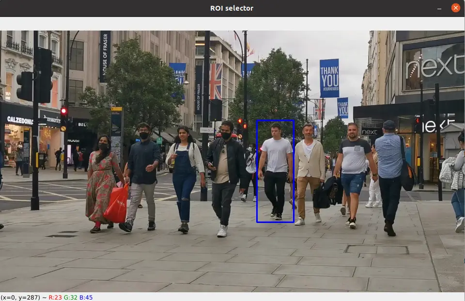
To manually select the object for tracking we call OpenCV function cv2.selectROI on Line 36 (you will see the window for manual selection) and initialize our tracker with this information on Line 37.

To update the location of the object we call the .update() method for our frame on Line 46. Next, in the loop, our tracker will process the video frame by frame and save the results in the video file until we stop the loop using commands on Lines 61-62.

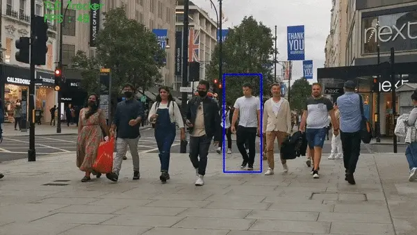
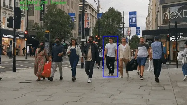
Now, let’s briefly consider each OpenCV object tracker methodology and look at the results we get.

Boosting Tracker

Boosting Tracker is based on the online version of the AdaBoost algorithm - the algorithm increases the weights of incorrectly classified objects, which allows a weak classifier to “focus” on their detection.

Since the classifier is trained “online”, the user sets the frame in which the tracking object is located. This object is initially treated as a positive result of detection, and objects around it are treated as the background.

Receiving a new image frame, the classifier scores the surrounding detection pixels from the previous frame and the new position of the object will be the area where the score has the maximum value.

Pros: an object is tracked quite accurately, even though the algorithm is already outdated.

Cons: relatively low speed, strong susceptibility to noise and obstacles, and the inability to stop tracking when the object is lost.

MIL (Multiple Instance Learning) Tracker

MIL Tracker has the same approach as BOOSTING, however, instead of guessing where the tracked object is in the next frame, an approach is used in which several potentially positive objects, called a “bag”, are selected around a positive definite object. A positive “bag” contains at least one positive result.

Pros: more robust to noise, shows fairly good accuracy.

Cons: relatively low speed and the impossibility of stopping tracking when the object is lost.

KCF (Kernelized Correlation Filters) Tracker

KCF Tracker is a combination of two algorithms: BOOSTING and MIL. The concept of the method is that a set of images from a “bag” obtained by the MIL method has many overlapping areas. Correlation filtering applied to these areas makes it possible to track the movement of an object with high accuracy and to predict its further position.

Pros: sufficiently high speed and accuracy, stops tracking when the tracked object is lost.

Cons: inability to continue tracking after the loss of the object.

TLD (Tracking Learning Detection) Tracker

TLD Tracker allows you to decompose the task of tracking an object into three processes: tracking, learning and detecting. The tracker (based on the MedianFlow tracker) tracks the object, while the detector localizes external signs and corrects the tracker if necessary. The learning part evaluates detection errors and prevents them in the future by recognizing missed or false detections.

Pros: shows relatively good results in terms of resistance to object scaling and overlapping by other objects.

Cons: rather unpredictable behavior, there is the instability of detection and tracking, constant loss of an object, tracking similar objects instead of the selected one.

Median Flow Tracker

Median Tracker is based on the Lucas-Kanade method. The algorithm tracks the movement of the object in the forward and backward directions in time and estimates the error of these trajectories, which allows the tracker to predict the further position of the object in real-time.

Pros: sufficiently high speed and tracking accuracy, if the object isn’t overlapped by other objects and the speed of its movement is not too high. The algorithm quite accurately determines the loss of the object.

Cons: high probability of object loss at high speed of its movement.

GOTURN (Generic Object Tracking Using Regression Network) Tracker

GOTURN Tracker algorithm is an “offline” tracker since it basically contains a deep convolutional neural network. Two images are fed into the network: “previous” and “current”. In the “previous” image, the position of the object is known, while in the “current” image, the position of the object must be predicted. Thus, both images are passed through a convolutional neural network, the output of which is a set of 4 points representing the coordinates of the predicted bounding box containing the object. Since the algorithm is based on the use of a neural network, the user needs to download and specify the model and weight files for further tracking of the object.

Pros: comparatively good resistance to noise and obstructions.

Cons: the accuracy of tracking objects depends on the data on which the model was trained, which means that the algorithm may poorly track some objects selected by the user. Loses an object and shifts to another if the speed of the first one is too high.

MOSSE Tracker

MOSSE Tracker is based on the calculation of adaptive correlations in Fourier space. The filter minimizes the sum of squared errors between the actual correlation output and the predicted correlation output. This tracker is robust to changes in lighting, scale, pose, and non-rigid deformations of the object.

Pros: very high tracking speed, more successful in continuing tracking the object if it was lost.

Cons: high likelihood of continuing tracking if the subject is lost and does not appear in the frame.

CSRT Tracker

CSRT Tracker uses spatial reliability maps for adjusting the filter support to the part of the selected region from the frame for tracking, which gives an ability to increase the search area and track non-rectangular objects. Reliability indices reflect the quality of the studied filters by channel and are used as weights for localization. Thus, using HoGs and Colornames as feature sets, the algorithm performs relatively well.

Pros: among the previous algorithms it shows comparatively better accuracy, resistance to overlapping by other objects.

Cons: sufficiently low speed, an unstable operation when the object is lost.

We are a startup factory specializing in the development of high-tech Computer Vision technologies aimed at solving large and complex practical problems. We partner with entrepreneurs and bootstrapped founders on mutually beneficial terms, providing them with our expertise, know-how, resources, and investments to develop the product from 0 to 1.

Earlier, we wrote an article about how we invested in and developed the Computer Vision startup SeedMetrics. You can learn more about how we have been growing this company over the past few years.

If you are interested in what we do, we will be happy to learn more about your story.

Time to sum up

In this article, we have discussed general ideas of OpenCV object tracking algorithms and compared their performance on the video example. If you are still confused in the decision of what algorithm to choose, we suggest starting with KCF, MOSSE and CSRT object trackers. We hope this guide will lead you to better and faster solutions in your future work on object tracking.