Creating a simple neural network in Python
Python is commonly used to develop websites and software for complex data analysis and visualization and task automation.
Today we’ll create a very simple neural network in Python, using Keras and Tensorflow to understand their behavior. We’ll implement an XOR logic gate and we’ll see the advantages of automated learning to traditional programming.
In our daily life, there are problems we know the logical steps to solve that we can describe in any programming language, but what happens when you don’t know the steps but instead you can see the input and outputs and see the problem as a black box? Then you can model this problem as a neural network, a model that will learn and will calibrate itself to provide accurate solutions.
To understand how it works, let’s dive into more details:
Requirements
You can just read the code and understand it but if you want to run it you should have a Python development environment like Anaconda to use the Jupyter Notebook, it also works with the python command line.
The logic XOR gate
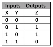
For the example, we’ll use the XOR gate. If you don’t remember them or just don’t know what’s that we’ll show you.
We have two binary entries ( 0 or 1) and the output will be 1 only when just one of the entries is 1 and the other is 0. It means that from the four possible combinations only two will have 1 as output.
The network
This is the code for this study case, later on, we’ll analyze the code step by step.
import numpy as np
from keras.models import Sequential
from keras.layers.core import Dense

training_data = np.array([[0,0],[0,1],[1,0],[1,1]], "float32")
target_data = np.array([[0],[1],[1],[0]], "float32")

model = Sequential()
model.add(Dense(16, input_dim=2, activation='relu'))
model.add(Dense(1, activation='sigmoid'))
model.compile(loss='mean_squared_error',
                       optimizer='adam',
                       metrics=['binary_accuracy'])
model.fit(training_data, target_data, epochs=1000)
scores = model.evaluate(training_data, target_data)

print("\n%s: %.2f%%" % (model.metrics_names[1], scores[1]*100))
print (model.predict(training_data).round())
Keras and Tensorflow
Let’s use Keras, a high-level library, to make easier the job of describing the layers of our network and the engine that will run and train the network is Google’s Tensorflow which is the best implementation we have available nowadays.
Analyzing the code
First, we need to import the classes we will use
import numpy as np
from keras.models import Sequential
from keras.layers.core import Dense
Numpy will be used for the management of arrays. From Keras we import the Sequential model and the Dense layer type which is the usual one. After this let’s create the input and output arrays
training_data = np.array([[0,0],[0,1],[1,0],[1,1]], "float32")
As you see, these are the combinations of the XOR and the expected results in the same order
target_data = np.array([[0],[1],[1],[0]], "float32")
Now is time to create the architecture of our neural network
model = Sequential()
model.add(Dense(16, input_dim=2,
                    activation='relu'))
model.add(Dense(1, activation='sigmoid'))
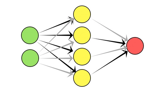
Here we create an empty model of type Sequential, which means our layers will be one after the other. Then we add two Dense layers with the model’s add method. It is actually three layers we are adding because by specifying input_dim = 2 it means we defined the input layer with two neurons, for our XOR input values. Our first hidden layer has 16 neurons. As an activation function, we use “relu” because we know it gives good results. You can set up your network as you want, this is just an example, there are off course, well-defined architectures but you can be creative for one time and explore by changing the number of layers, the activation function, and the number of neurons. Finally, we add the output layer with one node that will hold the result value with a sigmoid activation function.
Let’s train it
Before training the network we have to make some adjustments
model.compile(loss='mean_squared_error',optimizer='adam',metrics=['binary_accuracy'])
Here we define the loss type we’ll use, the weight optimizer for the neuron’s connections, and the metrics we need.
Now is time to train the net. Using the fit method we indicate the inputs, outputs, and the number of iterations for the training process. This is just a simple example but remember that for bigger and more complex models you’ll need more iterations and the training process will be slower.
model.fit(training_data, target_data, epochs=1000)
Training results
Let’s check the training outputs
Epoch 1/10004/4 [==============================] - 0s 43ms/step - loss: 0.2634 - binary_accuracy: 0.5000
Epoch 2/10004/4 [==============================] - 0s 457us/step - loss: 0.2630 - binary_accuracy: 0.2500
We can see it was kind of luck the firsts iterations and accurate for half of the outputs, but after the second it only provides a correct result of one-quarter of the iterations. Then, in the 24th epoch recovers 50% of accurate results, and this time is not a coincidence, is because it correctly adjusted the network’s weights.
Epoch 24/1000 4/4 [==============================] - 0s 482us/step - loss: 0.2549 - binary_accuracy: 0.5000
Epoch 107/1000 4/4 [==============================] - 0s 621us/step - loss: 0.2319 - binary_accuracy: 0.7500
Epoch 169/1000 4/4 [==============================] - 0s 1ms/step - loss: 0.2142 - binary_accuracy: 1.0000
And, in my case, in iteration number 107 the accuracy rate increases to 75%, 3 out of 4, and in iteration number 169 it produces almost 100% correct results and it keeps like that ‘till the end. As it starts with random weights the iterations in your computer would probably be slightly different but at the end, you’ll achieve the binary precision, which is 0 or 1.
Evaluation and prediction
First, we evaluate the model.
scores = model.evaluate(training_data, target_data)
print("\n%s: %.2f%%" % (model.metrics_names[1], scores[1]*100))
Then we see we achieved 100% accuracy, keeping in mind the simplicity of the example. And we make the 4 possible predictions for the XOR passing the entries.
print (model.predict(training_data).round())
Tuning the parameters of the network
This is a very simple example with only 4 possible entries but we can have a really complex network and it’ll be necessary to adjust the network's parameters like:
- Amount of layers
- Amount of neurons per layer
- Activation function per layer
- When compiling the model, the loss functions, the optimizer, and metrics
- A number of training iterations.
I recommend you to play with the parameters to see how many iterations it needs to achieve the 100% accuracy rate. There are many combinations of the parameters settings so is really up to your experience and the classic examples you can find in “must read” books.
Conclusion
Obviously, you can code the XOR with a if-else structure, but the idea was to show you how the network evolves with iterations in an-easy-to-see way. Now that you’re ready you should find some real-life problems that can be solved with automatic learning and apply what you just learned.

