
Twitter Sentiment Analysis in Python using Transformers
Twitter is a social media platform, and its analysis can provide plenty of useful information. In this article, we will show you, using the sentiment140 dataset as an example, how to conduct Twitter Sentiment Analysis using Python and the most advanced neural networks of today - transformers.
Transformers
Transformers technology was created in 2017, and since then, models based on it are the most popular and widely used. Earlier, we gave a detailed overview of transformers in Computer Vision. Today we will be using one of the main transformer-based models, the Robustly Optimized BERT Pre-training Approach (RoBERTa).
About RoBERTa
The RoBERTa model was proposed in RoBERTa: A Robustly Optimized BERT Pretraining Approach by Yinhan Liu, Myle Ott, Naman Goyal, Jingfei Du, Mandar Joshi, Danqi Chen, Omer Levy, Mike Lewis, Luke Zettlemoyer, Veselin Stoyanov. It is based on Google’s BERT model released in 2018.
It builds on BERT and modifies key hyperparameters, removing the next-sentence pre-training objective and training with larger mini-batches and learning rates.
Twitter Sentiment Analysis
Now that we know the basics, we can start the tutorial. Here's what we need to do to train a sentiment analysis model:
- Install the transformers library;
- Download the ROBERTA model and train for fine-tuning;
- Process the sentiment140 dataset and tokenize it using the Roberta tokenizer;
- Make predictions with the refined model and see when the model makes the wrong predictions.
We will use the ROBERTA model from the Transformers library, and use PyTorch as the main framework.
Install the Transformers Library
To install the Transformers library, simply run the following pip line on a Google Colab cell:
!pip install transformers
After the installation is completed, we will import the torch to add some layers for fine-tuning, Roberta's model, and Roberta's tokenizer. After that, we will create a model class, where we load the pre-trained model and add new layers:
import torch
from transformers import RobertaModel

class RobertaClass(torch.nn.Module):
    def __init__(self):
        super(RobertaClass, self).__init__()
        self.l1 = RobertaModel.from_pretrained("roberta-base")
        self.pre_classifier = torch.nn.Linear(768, 768)
        self.classifier = torch.nn.Linear(768, 2)

    def forward(self, input_ids, attention_mask, token_type_ids):
        output_1 = self.l1(input_ids=input_ids,
                           attention_mask=attention_mask,
                           token_type_ids=token_type_ids)
        hidden_state = output_1[0]
        pooler = hidden_state[:, 0]
        pooler = self.pre_classifier(pooler)
        pooler = torch.nn.Tanh()(pooler)
        output = self.classifier(pooler)
        return output

model = RobertaClass()
model.to(device)
“sentiment140” dataset
For our research, we will use this dataset.
The dataset consists of a table with 6 columns, we will use only 2 of them: “text” and “label” containing the tweet and the target label respectively. The volume of the dataset is 1.6 million tweets with 800 thousand positive and 800 thousand negative examples, i.e. the data is already perfectly balanced. The lengths of the tweets are distributed as follows:

As we can see, tweets longer than 140 characters can be discarded as statistically insignificant.
Also since a dataset with a volume of 1.6M is excessively large for a fine-tuned RoBERTa, we take only 100k of each type.
Let’s Load the Dataset
We will load the dataset from Google Drive, and for this, we will use the corresponding Google Drive library:
from google.colab import drive
# connect with your google drive
drive.mount('/content/drive')

import pandas as pd
# paste your path to the dataset
!cp '/content/drive/MyDrive/dataset.zip' dataset.zip
We need to unzip files from the archive:
import zipfile
with zipfile.ZipFile("dataset.zip", 'r') as zip_ref:
    zip_ref.extractall("./")
Preparing the Data
Let’s drop unnecessary columns and rename the remaining ones:
full_data = pd.read_csv('/content/training.1600000.processed.noemoticon.csv',
                        encoding='latin-1').drop(["1467810369",
                                                  "Mon Apr 06 22:19:45 PDT 2009",
                                                  "NO_QUERY","_TheSpecialOne_"],
                                                 axis=1).dropna()
columns_names = list(full_data)
full_data.rename(columns={columns_names[0]:"label",
                        columns_names[1]:"text"}, inplace= True)
In the dataset, positive tweets are marked with the number 4, but RoBERTa will perceive the number 4 as if we were predicting 5 classes or more. Since we only have two classes, we will have to replace the labels:
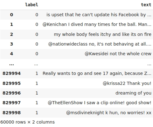
NUM_SAMPLES = 30000
negative_samples = full_data[full_data["label"]==0][:NUM_SAMPLES]
positiv_samples = full_data[full_data["label"]==4][:NUM_SAMPLES]

positiv_samples["label"]=[1]*NUM_SAMPLES

full_data = pd.concat([negative_samples,  positiv_samples])
We get the finished table:
Train and Test Split
We divide the sample into training and test splits. Don't forget to reset the indices:
from sklearn.model_selection import train_test_split
train_data, test_data = train_test_split(full_data, test_size=0.3)
train_data = train_data.reset_index(drop=True)
test_data = test_data.reset_index(drop=True)
positiv_samples["label"]=[1]*NUM_SAMPLES

full_data = pd.concat([negative_samples,  positiv_samples])
Tokenization
To process the text, we need to convert it into tokens. A special tokenizer is used for Roberta. It returns 3 values: a list of tokenized texts, a list of masks, and a list of token data types. After the tokenization, training and test data are stored in the train_tokenized_data and test_tokenized_data variables, respectively:
from transformers import RobertaTokenizer
tokenizer = RobertaTokenizer.from_pretrained('roberta-base',
                                             truncation=True,
                                             do_lower_case=True)
MAX_LEN = 130

train_tokenized_data = [tokenizer.encode_plus(
            text,
            None,
            add_special_tokens=True,
            max_length=MAX_LEN,
            pad_to_max_length=True,
            return_token_type_ids=True,
            truncation=True
        )
        for text in train_data['text']]

test_tokenized_data = [tokenizer.encode_plus(
            text,
            None,
            add_special_tokens=True,
            max_length=MAX_LEN,
            pad_to_max_length=True,
            return_token_type_ids=True,
            truncation=True
        )
        for text in test_data['text']]
Prepare dataset
Dataset class
For the convenience of using the data, we will create a dataset class, which will store all data for processing, targets, and source texts:
from torch.utils.data import Dataset, DataLoader
TRAIN_BATCH_SIZE = 32
TEST_BATCH_SIZE = 32
LEARNING_RATE = 1e-05

class SentimentData(Dataset):
    def __init__(self, data, inputs_tokenized):
        self.inputs = inputs_tokenized
        self.text = data['text']
        self.targets = data['label']

    def __len__(self):
        return len(self.text)

    def __getitem__(self, index):
        text = str(self.text[index])
        text = " ".join(text.split())

        input = self.inputs[index]
        ids = input['input_ids']
        mask = input['attention_mask']
        token_type_ids = input['token_type_ids']

        return {
            'sentence': text,
            'ids': torch.tensor(ids, dtype=torch.long),
            'mask': torch.tensor(mask, dtype=torch.long),
            'token_type_ids': torch.tensor(token_type_ids, dtype=torch.long),
            'targets': torch.tensor(self.targets[index], dtype=torch.float)
        }

train_dataset = SentimentData(train_data, train_tokenized_data)
test_dataset = SentimentData(test_data, test_tokenized_data)
Dataloader
Let’s put datasets in dataloader classes for taking the batches, and then shuffle them:
train_params = {'batch_size': TRAIN_BATCH_SIZE,
                'shuffle': True
                }

test_params = {'batch_size': TEST_BATCH_SIZE,
                'shuffle': True
                }

train_loader = DataLoader(train_dataset, **train_params)
test_loader = DataLoader(test_dataset, **test_params)
Fine-Tuning the RoBERTa Model
Now let's make a function for learning, and use it. During the training process, we will save the texts of the test data that the network will classify incorrectly:
from tqdm import tqdm
import matplotlib.pyplot as plt
from IPython.display import clear_output

train_loss = []
test_loss = []

train_accuracy = []
test_accuracy = []

test_answers = [[[],[]], [[],[]]]

def train_loop(epochs):
  for epoch in range(epochs):
    for phase in ['Train', 'Test']:
      if(phase == 'Train'):
        model.train()
        loader = train_loader
      else:
        model.eval()
        loader = test_loader
      epoch_loss = 0
      epoch_acc = 0
      for steps, data in tqdm(enumerate(loader, 0)):
        sentence = data['sentence']
        ids = data['ids'].to(device, dtype = torch.long)
        mask = data['mask'].to(device, dtype = torch.long)
        token_type_ids = data['token_type_ids'].to(device, dtype = torch.long)
        targets = data['targets'].to(device, dtype = torch.long)

        outputs = model.forward(ids, mask, token_type_ids)

        loss = loss_function(outputs, targets)

        epoch_loss += loss.detach()
        _, max_indices = torch.max(outputs.data, dim=1)
        bath_acc = (max_indices==targets).sum().item()/targets.size(0)
        epoch_acc += bath_acc

        if (phase == 'Train'):
          train_loss.append(loss.detach())
          train_accuracy.append(bath_acc)
          optimizer.zero_grad()
          loss.backward()
          optimizer.step()
        else:
          test_loss.append(loss.detach())
          test_accuracy.append(bath_acc)
          if epoch == epochs-1:
            for i in range(len(targets)):
              test_answers[targets[i].item()][max_indices[i].item()].append([sentence[i],
                                                                 targets[i].item(),
                                                                 max_indices[i].item()])

      print(f"{phase} Loss: {epoch_loss/steps}")
      print(f"{phase} Accuracy: {epoch_acc/steps}")
A long-awaited moment - we start to train our model. Since the model is not training from scratch, several epochs will be enough for us:
loss_function = torch.nn.CrossEntropyLoss()
optimizer = torch.optim.Adam(params =  model.parameters(), lr=LEARNING_RATE)

EPOCHS = 4
train_loop(EPOCHS)
Code for visualizing sentiment analysis
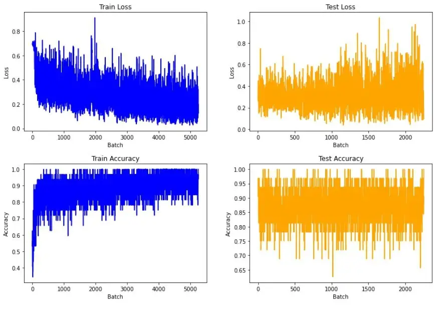
We will evaluate the results using graphs showing loss and accuracy:
plt.plot(train_loss,  color='blue')
plt.title("Train Loss")
plt.xlabel("Batch")
plt.ylabel("Loss")
plt.show()

plt.plot(test_loss,  color='orange')
plt.title("Test Loss")
plt.xlabel("Batch")
plt.ylabel("Loss")
plt.show()

plt.plot(train_accuracy,  color='blue')
plt.title("Train Accuracy")
plt.xlabel("Batch")
plt.ylabel("Accuracy")
plt.show()

plt.plot(test_accuracy,  color='orange')
plt.title("Test Accuracy")
plt.xlabel("Batch")
plt.ylabel("Accuracy")

plt.show()
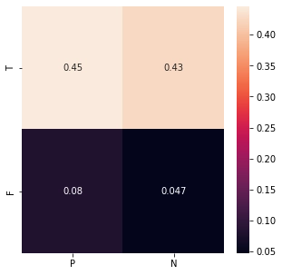
Here’s the confusion matrix:
import seaborn as sn
import pandas as pd
import matplotlib.pyplot as plt

len_num = len(test_dataset)

tp=len(test_answers[1][1])/len_num
fn=len(test_answers[1][0])/len_num
fp=len(test_answers[0][1])/len_num
tn=len(test_answers[0][0])/len_num

array_matrix = [[tp,tn],
                [fp,fn]]
df_cm = pd.DataFrame(array_matrix, index = ['T', 'F'],
                  columns = ['P', 'N'])
plt.figure(figsize = (5,5))
sn.heatmap(df_cm, annot=True)
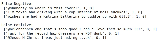
In the end, we will display wrongly predicted sentences:
print('False Negative:\n', test_answers[0][0][:3],
      'False Positive:\n', test_answers[0][1][:3])
Results
The model converges quickly to good values, and then converges much more slowly, changing its loss values in a limited range:
On the confusion matrix, we see that the model rarely makes mistakes, and often incorrectly predicts negative phrases, considering them positive:
Let's see in which predictions our network made a mistake. As we can see, only a few of them are real network errors. The rest of the errors are due to incorrect or controversial markup of the dataset:
Saving the Model
Finally, We can save our model to Google Drive:
save_path="./"
torch.save(model, save_path+'trained_roberta.pt')
print('All files saved')
print('Congratulations, you complete this tutorial')
Congratulations
You have successfully built a transformer classifier based on Roberta's model. Despite the not very high quality of the dataset, we managed to train the model to 87% accuracy, which is a great result in the task of tweet sentiment analysis. You can repeat the experiment with our Google Drive file.

