Intuitive Explanation of Meta-Learning

Introduction

Humans acquire many various concepts and skills over life. What important is that we are not learning them entirely from scratch but actively using past experiences. We use the skills we learned earlier when solving related problems as well as previously worked well approaches. The more experienced and skilled we are, the faster and easier it is for us to learn something new. To put it simply, we discover how to learn with experience.

The ability to learn and adapt quickly from a small number of examples is one of the most essential abilities of humans and intelligence in general. As opposed to humans, machine learning algorithms typically require a lot of examples to perform well. Thereby, the success of ML models has been mainly in areas where a vast amount of data can be collected or simulated. Such areas also have enormous compute resources available.

The question is how to obtain a good ML model in a situation when data is intrinsically rare or expensive or compute resources are unavailable? The standard answer is to use transfer learning. In transfer learning, we take a model trained on one or more large datasets and use it as starting points for training models on our small datasets.

For instance, we were asked to develop models to solve several medical tasks: task 1 - сlassification of tumors into benign and malignant on the image, task 2 - classify thoracic abnormalities from chest radiographs, task 3 - breast cancer detection, and so on. The problem is a critical lack of data: from 5 to 10 samples for each job. So we take a model pre-trained on the large ImageNet dataset and finetune it to each given task.

No doubt this approach often works well. However, the data on which the model has been pre-trained must have something in common with our data. Let's look at another approach for training models on a small amount of data - meta-learning.

Meta-Learning: An Intuition

Meta-learning provides an alternative paradigm where a machine learning model gains experience over multiple learning episodes – often covering the distribution of related tasks – and uses this experience to improve its future learning performance. In contrast, the conventional machine learning model gains knowledge only from data samples.

Going back to our example, let's say we have no pre-trained on the ImageNet initial parameters, but instead, we've randomly initialized them.

We'll train its model on its own dataset for each task, using random initial parameters θ as a starting point. Then, we evaluate models on their validation datasets. The smaller the error, the easier it is for the task to adapt initial parameters θ to its data. Using the validation errors (green lines on Fig 3.) of all tasks, we can measure how good the initial parameters θ were.

The next step is to answer the question, how can we find better initial parameters based on the information obtained? And the more interesting question is how to find such initial parameters that it would be easy to adapt them to the utterly new task using only a small number of training samples? There are many meta-learning methods for this, some of which we will discuss in the article.

You should note that meta-learning methods are not limited to finding the best initial parameters. Moreover, it is only a subset of a wide variety of meta-learning. Few categorizations of meta-learning can be found in the following surveys - [1], [2].

MAML

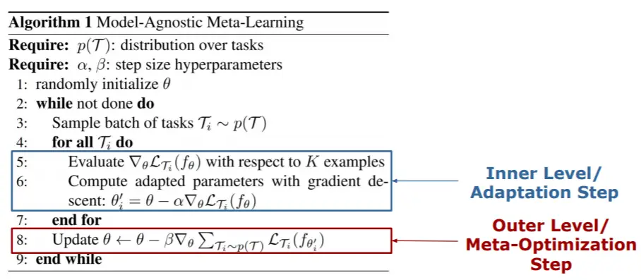
One of the notorious meta-learning algorithms is Model-Agnostic Meta-Learning (MAML) [3]. MAML finds the initialization of model parameters. That way, when given a new task, we can quickly and easily train a good model. We do it with only a couple number of gradient steps and a small amount of labeled data. Model-agnostic means that you can apply MAML to any model trained via gradient descent.

Suppose we are dealing with a supervised classification task T_1, and our model is f_θ with randomly initialized parameters θ. Using gradient descent steps, we can find optimal parameters that minimize the loss function for the given task.

Now let us have the distribution over similar tasks p(T). Meta-learning aims to find optimal parameters initialization from this distribution. It can be quickly adapted to a new related task using only a few labeled data and a few or even a single gradient step. To accomplish this, let's examine MAML in detail.

Initialization: A meta-model f_θ with randomly initialized parameters θ and distribution over similar tasks p(T).

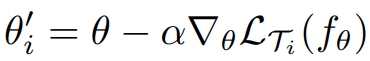
In general, MAML is a bi-level algorithm: in the Inner Level, we train a model for each task T_i and find corresponding optimal parameters θ_i. In the Outer Level, we update initial parameters θ of the meta-model f_θ.

Line 2: Sample a batch of tasks from the distribution over tasks p(T).

Lines 4 - 7: For each task T_i of the batch, we sample k training examples and obtain the corresponding optimal parameters θ_i from θ by one or more gradient descent steps.

Line 8: Perform meta-optimization via stochastic gradient descent: update initial parameters θ by calculating gradients with respect to the set of the optimal parameters from the previous step.

Meta-SGD

MAML finds the optimal initial parameters for the distribution over similar tasks. Meta-SGD [4] finds the update direction and learning rate, in addition to the optimal initial parameters. Mathematically, we do this by modifying Equation 1:

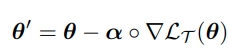
The difference is that learning rate α is a vector now and ◦ denotes element-wise product. In SGD, the learning rate is usually a small scalar value that decays over iterations. Instead, in Meta-SGD, we initialize the learning rate as a vector of shape θ with random values and learn them along with θ.

The update direction is represented by the vector α◦∇LT(θ) direction instead of the gradient direction ∇LT(θ). Learning rate implicitly implemented in the vector α◦∇LT (θ).

At the meta-optimization stage, we update initial parameters θ and also randomly initialized learning rate α (Line 9).

Reptile

We have to calculate second-order derivatives on the meta-optimization stage, which is not a computationally efficient task. To handle this issue, OpenAI proposed a modification of the MAML algorithm called Reptile [5].

In akin to MAML, Reptile is a model-agnostic algorithm that finds optimal parameter initialization to adapt to a new task quickly. But unlike MAML, Reptile does not require computation of the second-order derivatives directly.

Reptile consists of the following steps:

1. sample a batch of tasks,
2. training on it by multiple steps of the stochastic gradient descent,
3. move initial parameters θ towards optimal parameters obtained on the set of tasks from the previous step.

For instance, we've obtained new optimal parameters (Ws on the image) for two tasks. How do we move our initial parameters θ in a direction that's closer to both of these new optimal parameters? By minimizing Euclidean distance between initial and new optimal parameters.

Applications of Meta-Learning

Meta-learning methods are actively used in a wide variety of data science domains. For instance, in Computer Vision, they are used to handle different few-shot learning scenarios: few-shot multi-class classification, few-shot object detection, and segmentation, e.t.c. In Reinforcement Learning, meta-learning helps develop more "intelligent" agents who can learn new skills from small amounts of experience. In Neural Architecture Search, meta-learning helps to discover architectures that can generalize well to further problems.

Let's see how we can apply meta-learning to the tasks we covered in our blog earlier: face recognition and adversarial attacks on deep learning models.

Face Recognition with Meta-Learning

The paper [6] proposed a face recognition framework via meta-learning - Meta Face Recognition (MFR). In real-world face recognition applications, a situation may occur where the distributions between the source domains (on which the model was trained) and the target domains are very different. The deployed model should be able to generalize to unseen domains without any updating or finetuning. We can observe an example of such a situation during COVID-19: the quality of face recognition systems degrades significantly when the target domain consists of masked faces.

The idea is to simulate domain shifts within the source domains. Then, with meta-learning, we can obtain a model which generalizes well on target unseen domains without any finetuning.

MFR consists of three parts:

1. the domain-level sampling strategy for simulating domain shifts,
2. multi-domain distributions optimization to learn face representations,
3. the meta-optimization procedure to improve model generalization.

Domain-level Sampling

Let's suppose there are N source domains, and the goal is to simulate domain shifts that existed in real-world scenarios. We split N source domains into N-1 domains for meta-train and one target domain for meta-test during each training iteration. In the i-th iteration, the i-th source domain gets selected as the target domain. B identities are randomly chosen both from meta-train and meta-test domains. For each identity, two face images get chosen.

Optimizing Multi-Domain Distributions

Here, we optimize multi-domain distributions. The exact identities are mapped into nearby representations, and different identities are mapped apart from each other. There are three components:

1. Domain Alignment Loss learns to align domain centers.
2. Hard-pair attention loss focuses on optimizing hard positive and negative pairs.
3. Soft-classification Loss to perform classification within a batch

Thus, for each batch, we calculate the proposed losses for the meta-train domains:

Meta-optimization

What we've got so far: for each batch within the meta-batch, we sampled N−1 train domains and B pairs of images from it. Next, we calculated losses for meta-train domains. Now, we update the model parameters by gradient descent step:

This updated model then gets tested on the meta-test domain:

Finally, the final MFR objective is as follows:

By optimizing the model parameters, after updating the meta-train domains, the model also performs well on the meta-test domain. Once trained on source domains, you can directly deploy the model on target unseen domains.

Adversarial Attacks

Deep Neural Networks are vulnerable to adversarial attacks. An adversary can intentionally add hardly visual perturbation to the original input image. This causes the neural network to misclassify it. Recently, we examined some of the attack and defense methods in our blog.

Some works study the robustness of the Meta-Learning methods to the adversarially perturbed inputs. One of them is Adversarial Meta-Learning, where authors proposed a meta-learning algorithm ADML (ADversarial Meta-Learner). The idea is to combine MAML with Adversarial Training to enhance the robustness of a meta-model.

Likewise MAML, we have a meta-model f_θ with randomly initialized parameters θ.

At the inner level, the Fast Gradient Sign Method (FGSM) generates adversarial samples in addition to the clean training samples (Line 9). Thus, new model parameters are computed based on generated adversarial and clean samples (Line 10). Then (Line 12), generate another adversarial and clean samples for meta-update (meta-optimization).

At the outer level (Line 14), perform meta-update in an adversarial manner:

1. The gradient of the loss of the model updated using adversarial samples is calculated based on the clean samples (Line 14, green selection). Why is this needed? To make the model adapted to adversarial samples suitable also for clean samples.
2. The gradient of the loss of the model updated using clean samples is calculated based on the adversarial samples (Line 14, red selection). To make the model adapted to clean samples suitable also for adversarial samples.

The output of the ADML is an optimal initialization of model parameters θ, which is robust to adversarial samples. However, ADML is computationally expensive and challenging in optimization.

For those interested in adversarial attacks in the context of meta-learning, we highly recommend the following papers [8], [9].

Conclusion

To sum up, the goal of meta-learning is to train a model on various tasks. Such that it can solve new tasks using only a small number of training samples. This is very useful in real-world situations where we do not have large datasets for training. Or when we want to adapt our model to a new task quickly. We considered a category of meta-algorithms that tries to achieve this by finding a suitable initial parameter of the model that is well generalizable across related tasks. We looked at how we could apply these algorithms in the context of the tasks previously discussed in this blog.

References

[1] Hospedales T. et al. Meta-learning in neural networks: A survey //arXiv preprint arXiv:2004.05439. – 2020.

[2] Vanschoren J. Meta-learning: A survey //arXiv preprint arXiv:1810.03548. – 2018.

[3] Finn C., Abbeel P., Levine S. Model-agnostic meta-learning for fast adaptation of deep networks //International Conference on Machine Learning. – PMLR, 2017. – С. 1126-1135.

[4] Li Z. et al. Meta-SGD: Learning to learn quickly for few-shot learning //arXiv preprint arXiv:1707.09835. – 2017.

[5] Nichol A., Achiam J., Schulman J. On first-order meta-learning algorithms //arXiv preprint arXiv:1803.02999. – 2018.

[6] Guo J. et al. Learning meta face recognition in unseen domains //Proceedings of the IEEE/CVF Conference on Computer Vision and Pattern Recognition. – 2020. – С. 6163-6172.

[7] Yin C. et al. Adversarial meta-learning //arXiv preprint arXiv:1806.03316. – 2018.

[8] Goldblum M., Fowl L., Goldstein T. Adversarially robust few-shot learning: A meta-learning approach //arXiv preprint arXiv:1910.00982. – 2019.

[9] Wang R. et al. On Fast Adversarial Robustness Adaptation in Model-Agnostic Meta-Learning //arXiv preprint arXiv:2102.10454. – 2021.